While researching the difference between Intel’s various x86 SIMD extensions, I came across this article that demonstrates SSE and AVX performance differences using an algorithm to compute an approximation of pi using a Riemann sum under a curve. Specifically, we can numerically compute the integral
$$\int_{0}^{1} \frac{4}{1 + x^2} \mathrm{d} x = 4 \tan ^{-1} (x) = \pi $$
to find a reasonably quickly converging approximation of \( \pi \). This approach to approximating pi was novel to me, and seemed fun, so wrote a little Ink script to compute the integrals numerically for me.
The sum
If we wanted to establish upper and lower bounds for pi, we may take the left- and right-Riemann sums, but in this case I just wanted a useful approximation, so the approximation function computes the sum with each rectangle at the value of the midpoint of the rectangles’ base.
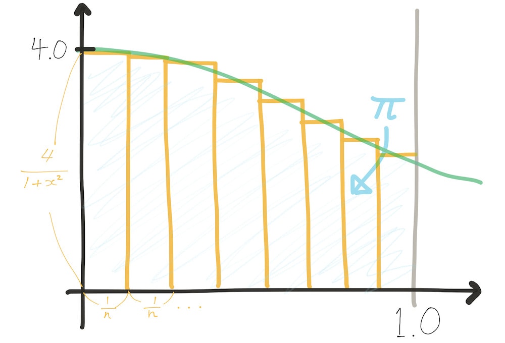
The sum we want to compute is just the sum of the areas of the \( n \) rectangles, expressed as
$$ \lim_{n \to \infty} \sum_{i = 0}^{n} \frac{1}{n} \frac{4}{1 + x_{i}^2} $$
where \( x_{i} \) is the midpoint of the base of the \( i \)-th rectangle of \( x \) between 0 and 1. Since \( x_{i} = \frac{1}{n} \cdot i + \frac{1}{2n} = \frac{2i + 1}{2n} \), we can rewrite the above as
$$ \pi = \lim_{n \to \infty} \sum_{i = 0}^{n} \frac{1}{n} \frac{4}{1 + \left( \frac{2i + 1}{2n} \right)^2} $$
which is the quantity our script will compute. In practice, we’ll write a program to compute this sum for some large values of \( n \).
The program
I started with an Ink script that simply computes the sum by applying the function
f := x => 4 / (1 + x * x)
over the values of range(0, 1, 1 / n) using the std.map function in the Ink standard library. But it turns out writing the algorithm using a single tail recursive function is much more efficient over iterating over a list, which brought me to this final version, which runs about 4x faster than the naive implementation I started with (~1.5 microseconds per rectangle vs. ~6μs).
` computing pi by integration
  from 0 to 1 of 4 / (1 + x ^ 2)
  as a Riemann sum `

` imports from the standard library `
std := load('std')
log := std.log
f := std.format
range := std.range
map := std.map

` estimation algorithm, given Count = n `
pi := Count => (
  ` memoized constants `
  Span := 1 / Count
  Span4 := 4 * Span
  HalfSpanSqAdd1 := Span * Span / 4 + 1

  ` inlined & optimized the function to integrate here
    where each column is fixed to the span's midpoint x-value `
  columnArea := x => Span4 / (x * (x + Span) + HalfSpanSqAdd1)

  ` sum the columns with a raw tail recursive loop `
  (sub := (x, acc) => x > 1 :: {
    true -> acc
    _ -> sub(x + Span, acc + columnArea(x))
  })(0, 0)
)
I tested the algorithm by computing the estimate at values of \( n \) from 100,000 up to 1,000,000.
` run estimate from 100k to 1M`

start := {time: time()}
K := 1000
M := K * K

map(
  ` for which values of n are we estimating? `
  range(100*K, 1*M+1, 100*K)

  count => (
    result := pi(count)

    end := time() `` time measurement for light profiling
    elapsed := floor((end - start.time) * 1000)
    start.time := end

    log(f(
      'Pi at Riemann sum of {{0}}: {{1}} ({{2}}ms)'
      [count, result, elapsed]
    ))
  )
)
I tested the script on my 2013 15" Macbook Pro, showing:
Pi at Riemann sum of 100000: 3.14161265 (155ms)
Pi at Riemann sum of 200000: 3.14159265 (295ms)
Pi at Riemann sum of 300000: 3.14159265 (451ms)
Pi at Riemann sum of 400000: 3.14159265 (592ms)
Pi at Riemann sum of 500000: 3.14159665 (738ms)
Pi at Riemann sum of 600000: 3.14159265 (892ms)
Pi at Riemann sum of 700000: 3.14159265 (1035ms)
Pi at Riemann sum of 800000: 3.14159515 (1172ms)
Pi at Riemann sum of 900000: 3.14159265 (1323ms)
Pi at Riemann sum of 1000000: 3.14159265 (1477ms)
which, while pretty slow to compute due to my language choice, is a respectable approximation of \( \pi \) for most practical uses.