
Until Elon Musk brings his Neuralink gadgets to market, our eyes are the highest-bandwidth way we have of understanding the world around us. We can look at something and immediately take in the hues, the lightness and the darkness, the shapes, and most importantly, the patterns that we wouldn’t be able to notice if we couldn’t use our vision.
In fact, our eyes are surprisingly good at pattern recognition, noticing the rhythm in the details that make up the large-scale structure of what’s in front of us. Today, I thought I’d put this to good use by trying to use our eyes’ pattern-noticing powers to get a more intuitive understanding of popular sorting algorithms in computer science. The header image for this post, for example, is a rendering of the popular quicksort algorithm, sorting from left to right. We’ll dig deeper into this at the end of this post.
A sorting algorithm, for the uninitiated, is a set of procedures that a computer program can apply repeatedly to take an “unsorted” list of items, like a list of numbers like [6, 41, 56, 7, 12], and transform it gradually into a fully sorted list, like [6, 7, 12, 41, 56]. Sorting algorithms are a well-trodden sub-branch of computer science, and there’s no shortage of fascinating visualizations and simulations online for studying these algorithms. So by no means are my renderings here completely novel, but I thought it was interesting nonetheless, and these images personally gave me a new level of intuitive understanding over these algorithms that I didn’t have before, even after having written them many times over. Let’s take a look at what’s going on.
The setup
I used Ink, a programming language I’m building from scratch, to write the program that generated these images. In the grand scheme of things, Ink isn’t the ideal language for something like this, but I thought it’d be a good way to find any bugs in my interpreter (I found none!), practice writing some sorting algorithms recursively, and exercise the language a little bit.
I wanted these images to allow me to easily, visually take in what a sorting algorithm did over time, as it took the list from an unsorted, random state to a completely sorted state. So I decided to imagine the image as a two-dimensional diagram. On the horizontal axis, we have a list of numbers, represented as a single line of colors. On the vertical axis, we represent time. As we travel down from the top of the image to the bottom of the image, we’ll take the list of numbers (the line of colored pixels) from a random ordering to a “sorted” rainbow line, by applying each kind of sorting algorithm one step per row. Here’s an example of what that looks like.
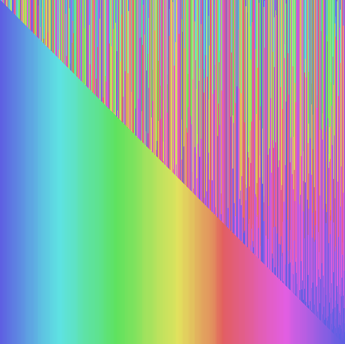
My particular implementation of this generates a list of 500 random numbers between 0 and 1, and at each line of pixels, I apply a single “step” of the algorithm, usually a single swap of two numbers in the list. And I continue adding on new lines until the “line” – the list – is completely sorted. The full program is a bit lengthy (about 340 lines), so I won’t embed it here, but you can find the Ink source code for this post on my GitHub, including the recursive implementations for all the algorithms we’ll explore here.
The algorithms
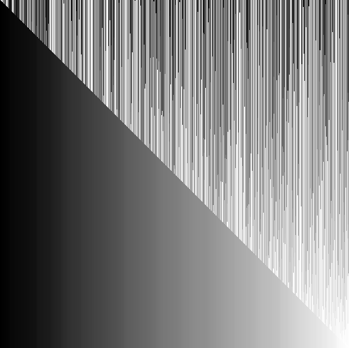
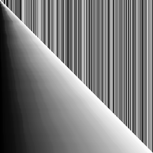
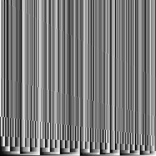
I rendered out the images for five common sorting algorithms in total: insertion sort, selection sort, bubble sort, merge sort, and quicksort. Let’s look at them in order. (I also linked under each image a greyscale version which conveys exactly the same information.)
Bubble sort
Of the five I rendered, bubble sort is the simplest and the slowest. Bubble sort goes like this:
- Start at the beginning of the list, and for each pair of numbers, if the first number is bigger than the second, swap their places.
- If you reach the end of the list, come back to the beginning and repeat.
- Repeat these steps until the list is completely sorted.
It turns out, this is a horrendously inefficient way to sort large lists of numbers. Even after vertically shrinking the generated image for bubble sort by 10 times, the only way I could fit it into this post was to lay it out horizontally, rotated by 90 degrees.
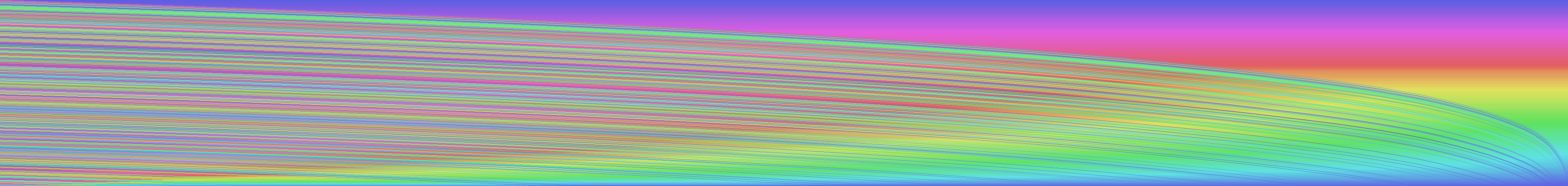
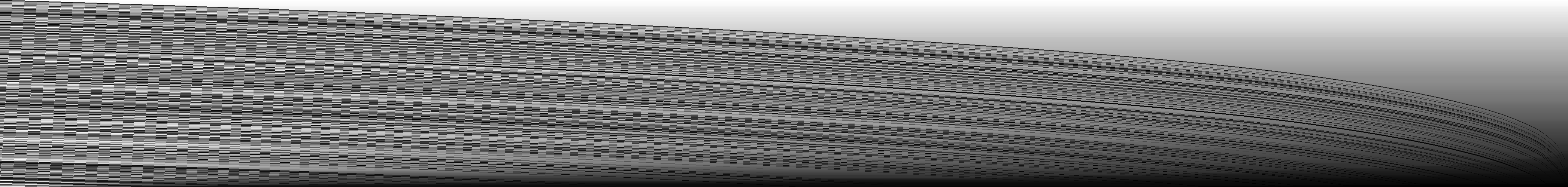
Here, we start with a random list on the left side of the image. Even though it isn’t obvious at all from the description of the algorithm, given the image, we can see exactly why this sort method is called “bubble” sort – the smallest numbers “bubble” up to the front of the list (the bottom of the image here) through time. We can also intuitively imagine why this algorithm takes so long to run to completion. The randomness in the initial list moves out slowly – each colored pixel takes many, many steps of bubble sort to find its correct place in the list.
Conclusion? Bubble sort is slow, but at least it’s got a fitting name.
Selection sort
The next algorithm I looked at is selection sort. Selection sort goes like this:
- Start at the beginning of the list
- Go through the list, one by one, to find the smallest item in the list, and move it to the front of the list
- Go through the rest of the list, to find the next smallest item in the list, and add it after the first item.
- Go through the rest of the list again, to find the next smallest item, and add it after the last one.
- Repeat this process until you’ve reached the end of the list.
Even though selection sort still seems radically simple, it turns out to be far more efficient than bubble sort. Here’s what it looks like.
You may notice that selection sort looks like a square. That’s not a coincidence – selection sort will, at worst, only swap as many times as there are items in the list, because it moves each item to its correct place in one swap operation, rather than moving things around haphazardly like bubble sort. This is what we call an O(n) algorithm – you can think of it as, for a list of n items, selection sort takes at most n steps to complete. This is why selection sort looks like a square – for 500 numbers, it took about 500 steps to finish.
I also noticed from this picture that selection sort builds up the final list in one smooth take, from the beginning of the list through to the end. Once the rainbow on the left side of the image starts forming, nothing is ever added to the left side or the inside of the rainbow – it only grows rightward. At each step, it just appends to the already-sorted section of the list. This makes it efficient in a way, because it doesn’t need to move a lot of numbers around – it just adds it to the end of a list each time. We’ll see in a minute that selection sort’s cousin, insertion sort, doesn’t share this property.
The last interesting property of selection sort is that, even partway through the sort process, a part of the list is completely sorted. This makes selection sort also a partial sort algorithm, which means that it can take a list and sort only a subset of it completely.
Insertion sort
Insertion sort is selection sort’s close cousin. It’s also got a square picture with an O(n) time complexity, and is fairly simple to describe. It goes like this:
- Start with the first number.
- For the number to the right of the first, if it’s less than the first, add it to the left of the first number; if it’s greater, add it to the right. We’ve just made a “sorted” subsection of our list with two numbers in it.
- For subsequent numbers we find on the right, find its correct place in our “sorted” section of the list on the left side, and insert the new number into its correct place.
- Continue doing this until you reach the right end of the list.
Insertion sort looks familiar, but it has one major difference.
The major difference is that, unlike selection sort, insertion sort isn’t a partial sort algorithm. It takes whatever number it finds as it goes through the list, and tries to sketch out the shape of the final list from the get-go, adding each number it finds to the middle of the “sorted” section, the rainbow.
Because of this, insertion sort involves a bit more shuffling of numbers than selection sort. When we find, say, a yellow number halfway through our sort, we have to insert the number into the middle of our sorted section – the rainbow half – and shift all the remaining numbers one place to the right. This is a contrast against selection sort, where we simply add numbers to the right end of the sorted sub-list. However, this is outweighed by a benefit of insertion sort – because we look for a place for each new number within the smaller, sorted subsection of the list, rather than when trying to find the minimum of the whole remaining list, we perform fewer comparisons with each number in each sort step. On balance, this can sometimes make insertion sort faster in practice than selection sort.
However, none of these algorithms so far are a match for the two remaining ones, which are much more efficient on large lists.
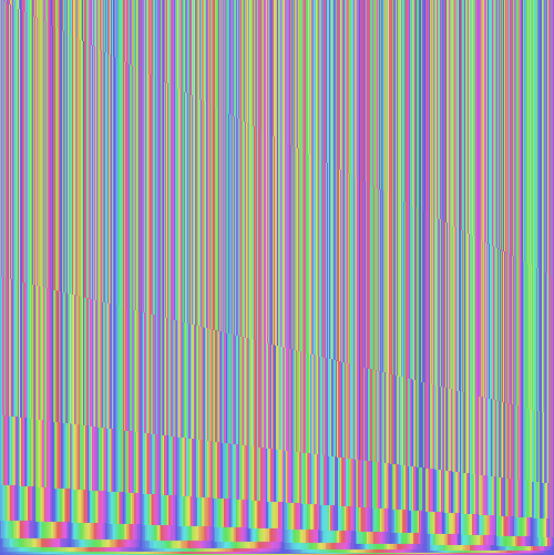
Merge sort
Merge sort, and its relative quicksort, have more complex implementations that are harder to describe precisely in words. Merge sort’s general idea is that we divide the list into smaller and smaller subsections, sort the smaller sections, and then “merge” those smaller, already sorted subsections of the list while preserving the order of the numbers in it. It looks like this.
I was surprised to see that it doesn’t feel like merge sort has a lot of “sorting” going on for most of its time – for most of the image, the list looks pretty random. But towards the end (the bottom), we start to see these sorted subsections more clearly, as they appear as smaller rainbows that “merge” into larger ones, until they form a single long rainbow line at the bottom of the image. This is merge sort in action. If you look closer, you can see some faint streaks in the middle as tiny 2- and 4-element subsections are sorted and then merged into larger subsections.
Although I’ve formatted the image here as a square for convenience, merge sort is actually much faster in practice for long lists than any of the algorithms we’ve encountered so far – when a list doubles in size, we only need to do about twice as much work, rather than re-reading a doubly large list many times over, as we’d have to do in other sorting algorithms above. One last notable property of merge sort is that different sections of a list can be merge-sorted in parallel. This means, if you have multiple computers or multiple CPU cores in a single computer, you may be able to share the work of merge-sorting very, very large lists rather efficiently. (Modern computers are fast enough that, in practice, this is usually irrelevant.)
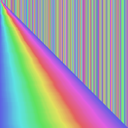
Quicksort
Quicksort is the most popular sorting algorithm among the ones we’re looking at today. Most languages’ baseline sort operations implement quicksort under the hood, including the standard C library’s gsort() and JavaScript’s Array.prototype.sort(). It’s so popular because it’s rather efficient, more so than the other four in this list. Quicksort is a mouthful to explain in detail, but all you need to know, if you don’t already, is that quicksort, like merge sort, depends on an approach of splitting up a list into ever smaller parts to be sorted again.
Its portrait is also the most interesting in my opinion.

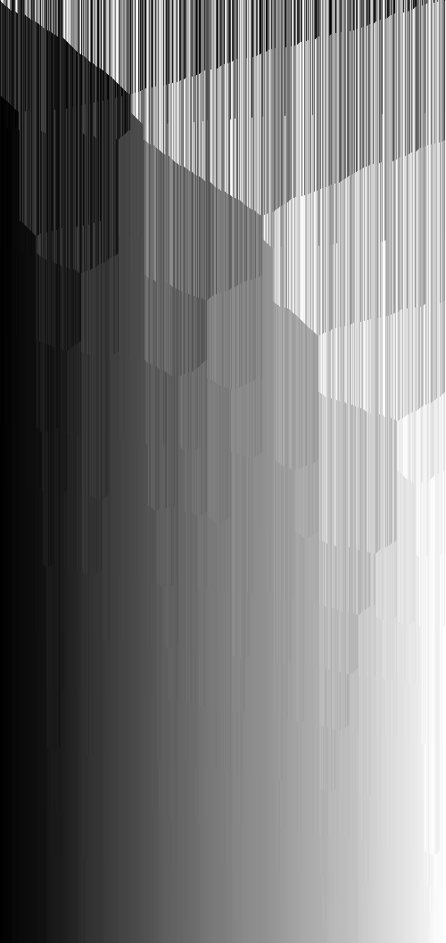
In this picture of quicksort, we can clearly see where the sorted subsections are, and how they come together. Unlike merge sort, quicksort starts with very visible partitions. Quicksort starts by picking a number from the list, called a “pivot”, and splitting the list into two parts – the part with numbers less than the pivot, and the part with the numbers greater than it. In the picture, these appear at the top as the mostly-green and mostly-pink subsections of the top of the list.
This process repeats, until we get a cleanly sorted list at the end. Interestingly, the divisions are rarely exactly 50-50, as they were in merge sort. Instead, these divisions are arbitrary, and depend on the pivot point picked out for each divide. The way we pick these pivot points turns out to matter a lot in how efficient quicksort is for a given list. The more evenly split the partitions, the more efficient the resulting quicksort. In this example, we use a partition scheme by Tony Hoare, which proves efficient for most situations.
Wrapping up
Besides giving me a refresher on some of these algorithms, going through these generated images reminded me that sometimes, our eyes notice patterns that we can’t grasp just by staring at diagrams and words and code. I think representing algorithms as timelines or time “streaks” like these images can also be tremendously useful for teaching computer science concepts in general, beyond sorting algorithms.
There’s a multitude of sorting algorithms that researchers and engineers have invented over the years, and these five are just a taste of the variety in complexity and efficiency in the landscape. If you’re interested in the topic, definitely give the Wikipedia article on sorting algorithms a once-over, and look around for other interesting data visualizations and interactive demos around sorting algorithms elsewhere on the web – there’s plenty.
And as it goes without saying, if you’re interested in the code for these particular images or for the Ink programming language, check out my GitHub and Twitter, where you can usually follow updates.